Statistically most probable stoichiometric formulae

     W. A. DOLLASE AND W. I. NEWMAN

     Department of Earth and Space Sciences

University of California, Los Angeles

Los Angeles, California 90024

     Abstract

A method of calculating the most probable chemical formula of a compound from its measured (and therefore inaccurate) chemical analysis is presented. The method, which uses a Lagrange multiplier technique, allows testing of the hypothesis that a given analysis conforms to specific formula constraints. An example involving ferrous/ferric ratio estimation is given.

     Introduction

     It is commonly useful to determine the stoichiometric formula of a mineral from its chemical analysis. If this analysis were both perfectly accurate and complete for all elements, such recalculation would be unambiguous. However, real analyses as obtained for example with an electron microprobe, are neither perfect nor complete. The problem of obtaining the "true" formula from incomplete or inaccurate data can be visualized geometrically. The measured chemical analysis of a mineral containing n elements is representable as a point in an n-dimensional space where each coordinate axis represents the concentration of one of the elements in the mineral. All points in this space, however, do not yield possible or probable formulae, that is, the analysis point may recalculate to a formula which has an impossible or improbable ratio of total anions to total cations, or atoms in tetrahedral sites to atoms in octahedral sites, etc. The locus of all possible or permissible elemental concentrations forms a subspace contained within this n-dimensional analysis space having the property that all points on this subspace conform exactly to a set of specified stoichiometric formula constraints. In order to emphasize the geometric conception of this method, it is convenient to think of this subspace as a surface imbedded within the n-dimensional volume. As the measured analysis point does not in general fall on this surface, the problem is to find that point on the stoichiometric surface which is "nearest" (in a least squares sense) the measured analysis point. This nearest point on the stoichiometric surface yields the statistically most probable formula while the distance between the analysis point and the nearest stoichiometric point carries information regarding the probability that this analysis conforms to the specified stoichiometry.

     Method of solution

     Let Y₁, ...,Y_n represent the measured concentrations of the n elements (or more generally, oxide components) and X₁, . ..,X_n represent the corresponding concentrations of the stoichiometric analysis point nearest the measured analysis point. The sum of the squares of the differences between the X's and corresponding Y's is a measure of the distance between these points. However, in order to combine data for several elements it is necessary to express the differences between measured and theoretical concentrations in terms of the number of measurement standard deviations this difference represents. Thus the appropriate distance (squared) between the measured analysis point and the nearest stoichiometric analysis point is given by:

where σ_i is the standard deviation in the measurement of the concentration of element i. The problem is to choose values of X which minimize U but also conform to all stoichiometric constraints. The method of Lagrange multipliers is well suited to this type of optimization and can be used here (e.g., Hildebrand, 1965, p. 120).

     The constraints on a chemical formula can be written as a series of m linear equations in terms of the concentrations of the elements present. Thus for the j-th constraint, j = 1, ...,m):

where N_i is the number of atoms of type i in the formula, the C_j,i's are the constraint coefficients and C_j,o is the constraint sum. For example, in the case of plagioclase the following equations can be written:

     8=0.5N_Na+1.0N_Ca+1.5N_Al+2.0N_Si 
       4=0.0N_Na+0.0N_Ca+1.0N_Al+1.0N_Si 
       1=1.0N_Na+1.0N_Ca+0.0N_Al+0.0N_Si 

     These particular equations specify that in the ideal plagioclase formula there are eight total oxygens, four atoms in tetrahedral sites, and that the sum of Na + Ca is equal to one. If an element such as potassium is also present an additional term can be added to each constraint equation, and so forth.

     The number of atoms per formula unit is related to the oxide component concentrations, Xi by:

     N_i = k X_i/W_i, (3)

where W_i is the molecular weight (per metal atom) of the i-th oxide and k is a normalization constant that is to be determined. Thus for the j-th constraint, (j = 1, ...,m):

In addition to these constraints, an equation stating that the sum of the components is equal to unity can be written:

For convenience, the presently unknown variable, 1/k, can be replaced by an ancillary variable, namely, X_n+1. In the Lagrange multiplier method the function to be minimized is:

where U is as defined above, the L_j are constants (Lagrange multipliers) whose values are to be determined and the h_j are the right hand sides of the constraint equations given above (equations (4) and (5)). Note that H is the (weighted) sum of the deviations between measured and stoichiometric concentrations plus the (weighted) sum of the constraint equations and that when the constraints are obeyed, all h_j = 0 and, under these conditions, H = U.

     The function H is minimized by setting each of the derivatives of H with respect to X_i, ..., X_n and to X_n+i = 1/k equal to zero. This in turn gives n equations of the form:

and one of the form:

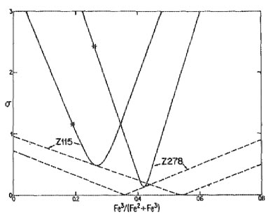
These n + 1 equations when added to the m + 1 constraint equations yield a total of n + m + 2 linear equations in n + m + 2 unknowns (the n values of X, the value of the normalization constant and the m + 1 Lagrange multiplier values). Provided this system of equations is not singular, it can be solved by conventional asymmetric matrix inversion methods to yield the desired concentrations and normalization constant.

     In addition to the concentrations and resulting most probable formula, this analysis provides a measure of the statistical likelihood that a particular analysis conforms to the particular set of formula constraints employed. Thus the quantity U from equation (1), or more conveniently the square root of the mean value of its component terms, rms U (referred to herein as the "rms analysis error"), is an index useful in hypothesis testing. Note that in this formulation it has been assumed that the measurement errors are independent of each other. An analysis which yields an rms analysis error on the order of one sigma or less is thus highly probable and is the normal expectation. On the other hand, an rms analysis error on the order of three sigma or more is rather improbable and indicates an unexpectedly large measurement error has occurred or that one or more of the hypothesized formula constraints is inappropriate.

Standard deviations

     The comparison of theoretical and measured concentrations requires a knowledge of the standard deviation of measurement for each element (or oxide component) present. In the absence of any systematic error these could be obtained by repeated analyses. In practice, since there no doubt are systematic errors present in concentration measurements, careful consideration of test data from well characterized standards may be needed to obtain appropriate measurement standard deviations. In the present treatment it has been found convenient to formulate the standard deviations as a linear function of concentration:

     σ_i=Y_i·(F_i-E_i)+E_i,   i=1,...,n,         (9)

where E_i and F_i are the estimated standard deviations for element i at concentrations of 0 and 1, respectively. E_i is comparable to the minimum detectable concentration under the analysis conditions and F_i is the rms analysis error that would be observed in analyses of pure component i.

Analysis concentration total

     Though frequently tabulated (and occasionally incorrectly used as the principal index of analysis quality), the sum of concentrations of components in an analysis usually has no influence on the resultant chemical formula no matter whether that total is 100% or 150%. This is, of course, because the formula represents only the ratios of elements present. However, the statistically most probable chemical formula may be influenced by the deviation from 100%.

Example of application

     The most probable stoichiometric formula calculations outlined above have been programmed and applied to numerous analyses. An example will serve to illustrate some of the applications of this technique. Miyano and Miyano (1982) have published electron microprobe analyses of ferri-annites from Western Australia. As they have not reported standard deviations of measurement for individual elements, values which are consistent with microprobe technology in general and their data in particular were estimated. The standard deviation of measurement of all elements was estimated as 1 wt.% at concentrations of 100% decreasing as a linear function of concentration to 0.05 wt.% at a concentration of 0%. Although no doubt incorrect in detail, and specifically violating the caution mentioned above, these estimates are adequate for demonstration purposes.

     A most probable formula analysis was applied in several steps. In the first step only the constraint of 22 total oxygens in the anhydrous formula was applied. The resulting cation proportions are then as reported by Miyano and Miyano in their Table 1 and 2. As a second step the analyses were constrained to total to 100% and H₂O was added as an analysis component. Because hydrogen was not measured, its concentration was entered as zero but its estimated error of measurement was entered as infinity. The first constraint was rewritten to give 24 total oxygens and the number of hydrogens was constrained to 4. If this latter constraint were not specified, the rms analysis error could be made zero by setting the H₂O content equal to the difference between the anhydrous total and 100%.

     In general, the analyses including this constrained amount of H₂O total slightly below 100%. The rms analysis errors are on the order of one standard deviation or less showing that the analyses largely fall within the assumed experimental errors. Furthermore, the generally small deviations from 100% totals can be removed by converting some of the presumed Fe²⁺ to Fe³⁺ because of the larger proportion of oxygens contributed by the latter species. This is illustrated by the dotted line curves in Figure 1 for typical analyses Z115 and Z278. At a ratio of Fe²⁺/(Fe²⁺+Fe³⁺) equal to 0.36 and 0.54, respectively, the analysis totals go to 100% thereby yielding calculated analyses that match the observed analyses exactly, that is the rms analysis error drops to zero. Note, however, that the slope of the dotted line curves is so low that essentially any ferric/ferrous ratio will give an acceptable rms analysis error. Thus, as is well known, the estimation of ferrous-ferric contents from analysis totals is generally too imprecise to be useful.

     In the next step, the sum of the cations in the tetrahedral plus octahedral sites was constrained to 14 (eight tetrahedral sites and six octahedral sites per 24 oxygen atom formula). Whether or not this constraint holds in individual micas is a subject of debate and will be tested here. As shown by previous authors (e.g., Finger, 1972) the ferric-iron proportion can be adjusted to give a prescribed cation/anion ratio. The solid line curves in Figure 1 show the rms analysis errors for these same two analyses under the assumption of this additional constraint. Note that these curves are much steeper than the dotted line curves and the location of the minimum can be used to estimate the ferric-iron proportion provided that the constraints which fix the cation/anion ratio are warranted. This in turn can be determined by the height of the minima in these curves. That is, using the assumed measurement standard deviations, the minimum rms analysis errors are much less than one sigma and therefore the assumption of full occupancy of the tetrahedral and octahedral sites is consistent with the analyses. The probable error in the ferric proportion estimated in this manner, is related to the steepness of the solid line curves. If a one sigma or less rms analysis error is considered probable, then the ferric-iron proportion is estimated to ±6% for these analyses. The asterisk shown on the solid line curves corresponds to the minimum ferric iron proportion estimated by Miyano and Miyano under the assumption "that all Fe³⁺, Al and Si are located on tetrahedral sites totalling 8 cations". That the minima occur at slightly higher ferric iron proportions indicates that an additional small proportion of the octahedrally coordinated iron atoms are also ferric species.

    
 Fig. 1. Rms analysis error versus ferric iron proportion for two ferri-annites calculated from measurements of Miyano and Miyano, 1982.

     As a last step it is possible to test the hypothesis of full occupancy of the interlayer sites in these micas by K + Na + Ca atoms. Inclusion of this additional constraint seems unwarranted, however, as the rms analysis errors then rise to generally over three standard deviations and the apparent error in the K₂O content rises to the highly improbable value of 8 sigma. Thus the deficiency of the interlayer site appears to be real, at least for these micas.

Acknowledgments

     We thank C. Ross for a review of the manuscript. 

References

     Finger, L. W. (1972) The uncertainty in the calculated ferric iron content of a microprobe analysis. Carnegie Institution of Washington Year Book, 71, 600-603.

     Hildebrand, F. B. (1965) Methods of Applied Mathematics, 2nd edition. Prentice-Hall, New Jersey.

     Miyano, T. and Miyano, S. (1982) Ferri-annite from the Dales Gorge Member iron-formations. American Mineralogist, 67, 1179-1194.

     Manuscript received, February 14, 1983; accepted for publication, October 24, 1983.